The Titanic data set is said to be the starter for every aspiring data scientist. So it was that I sat down two years ago, after having taken an econometrics course in a university which introduced me to R, thinking to give the competition a shot. My goal was to achieve an accuracy of 80% or higher.

However, my first try in this competition ended up with me producing some summary statistics and trying to solve the challenge with a linear regression model :). In short, I misinterpreted what the data science community meant by: “a competition for beginners”.

Now, two years later, I again tried my luck. Knowing about terms like training and testing data sets, overfitting, cross-validation, bias-variance trade-off, regular expressions, and about different classification models makes me hopefully better prepared this time. After almost having completed a Statistics degree, countless hours on Coursera, Data Camp and Stackoverflow, and after having a data science internship under my belt I finally declared myself a “beginner” in the data science community and ready for the Titanic Kaggle Competition.

Long story short, don’t be discouraged if you hear the words “beginner competition”, but are not yet able to understand everything or produce the results other people showcase in their kernels.

This blog post is an attempt to make the titanic data set easier to understand. Throughout it, I will be explaining my code.

What we will be covering in this blog post:

An Exploratory Data Analysis with ggplot2 and dplyr.
Feature Engineering for some Variables.
Dealing with Missing Values.
Model Building and Model Evaluation:
1. Logistic Regression
2. Random Forest
3. Linear Discriminant Analysis
4. K-Nearest Neighbors

In the end, I am ending up with a score of around 79%. Pretty disappointing for me and I didn’t achieve my initial goal of 80%. This is why in the second part of this tutorial, I evaluated the so-called gender model with which I achieved a score of 81.82%.

Let’s get started!

First, we are loading the libraries we need. The tidyverse consists of various packages (dplyr, ggplot, etc.) and is perfect for data manipulations. The ggbubr package is nice for visualizations and gives us some extra flexibility. The arsenal package is for easily creating some nice looking tables. The other packages are for building predictive models.

After having loaded the packages, we are loading the data sets. In order to rbind() them, the train and test data sets have to have equivalent columns. That is why I am creating the Survived column in the test data set. After that, I am transforming some variables with mutate() to characters and factors.

library(tidyverse) # data manipulation
library(ggpubr) # data visualization
library(arsenal) # table creation
library(randomForest) # model buliding
library(caret) # model building
library(class) # model building
library(MASS) # model building

#Loading and combining the data sets
train <- read.csv("train.csv")
test <- read.csv("test.csv")
test$Survived <- NA
titanic <- rbind(train, test) # combining data sets

# data manipulation
titanic %>%
  dplyr::mutate(
    Name = as.character(Name),
    Ticket = as.character(Ticket),
    Cabin = as.character(Cabin),
    Survived = as.factor(Survived),
    Pclass = as.factor(Pclass)
  ) -> titanic

Exploratory Data Analysis of the Titanic Data Set

Investigating Gender for the Titanic Data Set

For all my plots, I am using ggplot2. If you are unfamiliar with the syntax, the R for Data Science book, Data Camp, and the ggplot cheat sheet are great resources that you can refer to.

plot_count <- ggplot(titanic[1:891, ], aes(x = Sex, fill = Survived)) +
  geom_bar() +
  scale_fill_manual(
    name = "Survived",
    values = c("red", "blue"),
    labels = c("No", "Yes"),
    breaks = c("0", "1")
  ) +
  ggtitle("Most of the Titanic Passengers are Male.\n 
Most Passengers Who Survived Were Female") +
  theme(
    plot.title = element_text(hjust = 0.5),
    legend.position = "bottom"
  )

plot_percent <- ggplot(titanic[1:891, ], aes(x = Sex, fill = Survived)) +
  geom_bar(position = "fill") +
  scale_fill_manual(
    name = "Survived",
    values = c("red", "blue"),
    labels = c("No", "Yes"),
    breaks = c("0", "1")
  ) +
  ggtitle("75% of all Female Passengers Survived whereas only \n around 20% of the Male Passengers Survived") +
  theme(
    plot.title = element_text(hjust = 0.5),
    legend.position = "bottom"
  )

ggarrange(plot_count, plot_percent)

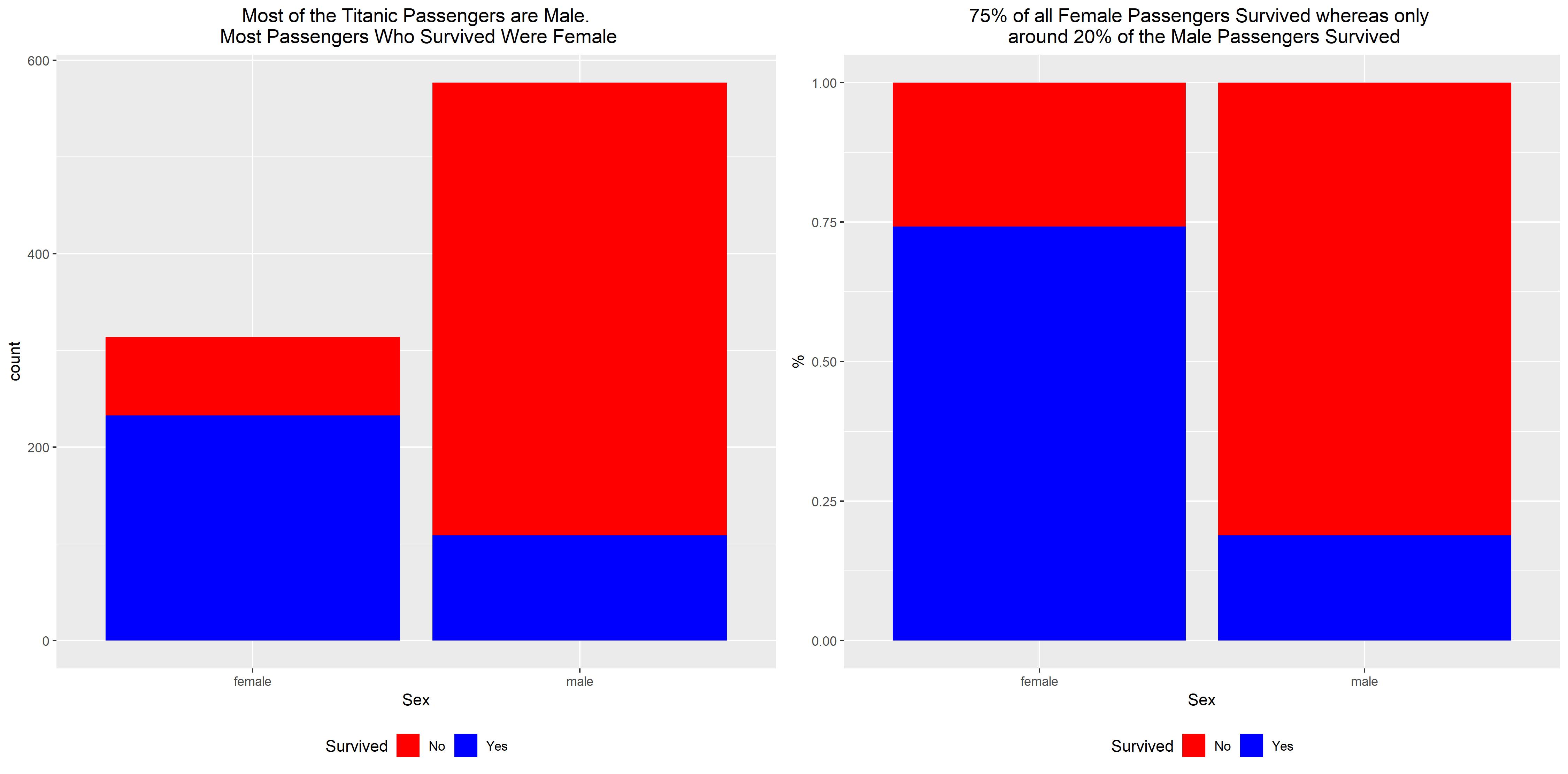
It looks like most of the female titanic passengers survived and most of the male passengers died. This becomes especially visible when looking at the percentages on the right plot. 75% of all female passengers survived whereas less than 25% of male passengers survived.

This is a very crucial finding and is key for the 81.82% success of the gender model I am discussing in part 2.

Investigating Gender and Class for the Titanic Data Set

plot_count <- ggplot(titanic[1:891, ], aes(x = Sex, fill = Survived)) +
  geom_bar() +
  facet_wrap(~Pclass) +
  scale_fill_manual(
    name = "Survived",
    values = c("red", "blue"),
    labels = c("No", "Yes"),
    breaks = c("0", "1")
  ) +
  theme(legend.position = "bottom")

plot_percent <- ggplot(titanic[1:891, ], aes(x = Sex, fill = Survived)) +
  geom_bar(position = "fill") +
  facet_wrap(~Pclass) +
  scale_fill_manual(
    name = "Survived",
    values = c("red", "blue"),
    labels = c("No", "Yes"),
    breaks = c("0", "1")
  ) +
  theme(legend.position = "bottom") +
  ylab("%")

combined_figure <- ggarrange(plot_count, plot_percent)
annotate_figure(combined_figure,
                top = text_grob("Almost All Female Passengers Who are Class One and Two Survived. The Big Proportion of Men not Surviving \n Mainly Comes From Male Class 3 Passengers",
                                color = "black",
                                face = "bold",
                                size = 14
                )
)

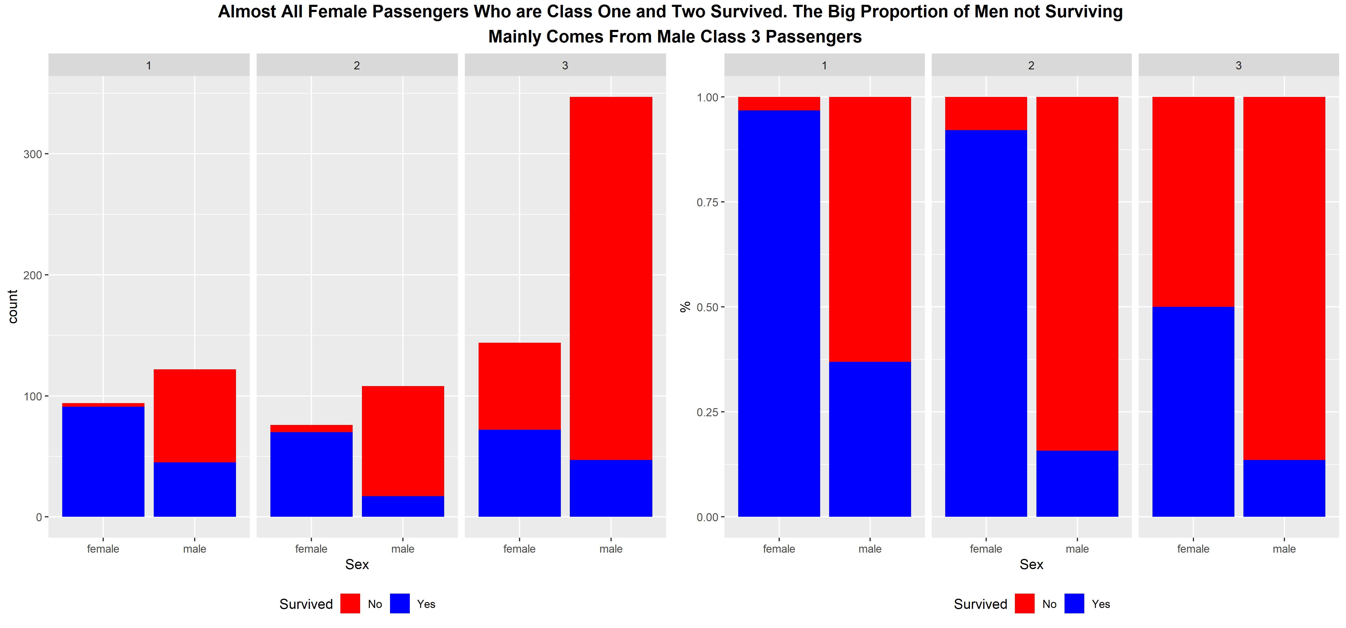
Almost all female passengers in classes 1 and 2 survived whereas, for males, the passenger class is not a great predictor for survival. This is because regardless of class, male passengers do not really seem to benefit much from being in higher classes.

Investigating Age, Fare, and Embarked for the Titanic Data Set

plot_age <- ggplot(titanic[1:891, ], aes(x = Age, fill = Survived)) +
  geom_histogram() +
  scale_fill_manual(
    name = "Survived",
    values = c("red", "blue"),
    labels = c("No", "Yes"),
    breaks = c("0", "1")
  ) +
  theme(legend.position = "bottom")

plot_fare <- ggplot(titanic[1:891, ], aes(x = Fare, fill = Survived)) +
  geom_histogram() +
  scale_fill_manual(
    name = "Survived",
    values = c("red", "blue"),
    labels = c("No", "Yes"),
    breaks = c("0", "1")
  ) +
  theme(legend.position = "bottom")

plot_embarked <- ggplot(titanic[1:891, ], aes(x = Embarked, fill = Survived)) +
  geom_bar() +
  scale_fill_manual(
    name = "Survived",
    values = c("red", "blue"),
    labels = c("No", "Yes"),
    breaks = c("0", "1")
  ) +
  theme(legend.position = "bottom")

ggarrange(plot_age, 
          plot_fare, 
          plot_embarked, common.legend = TRUE, ncol = 3)

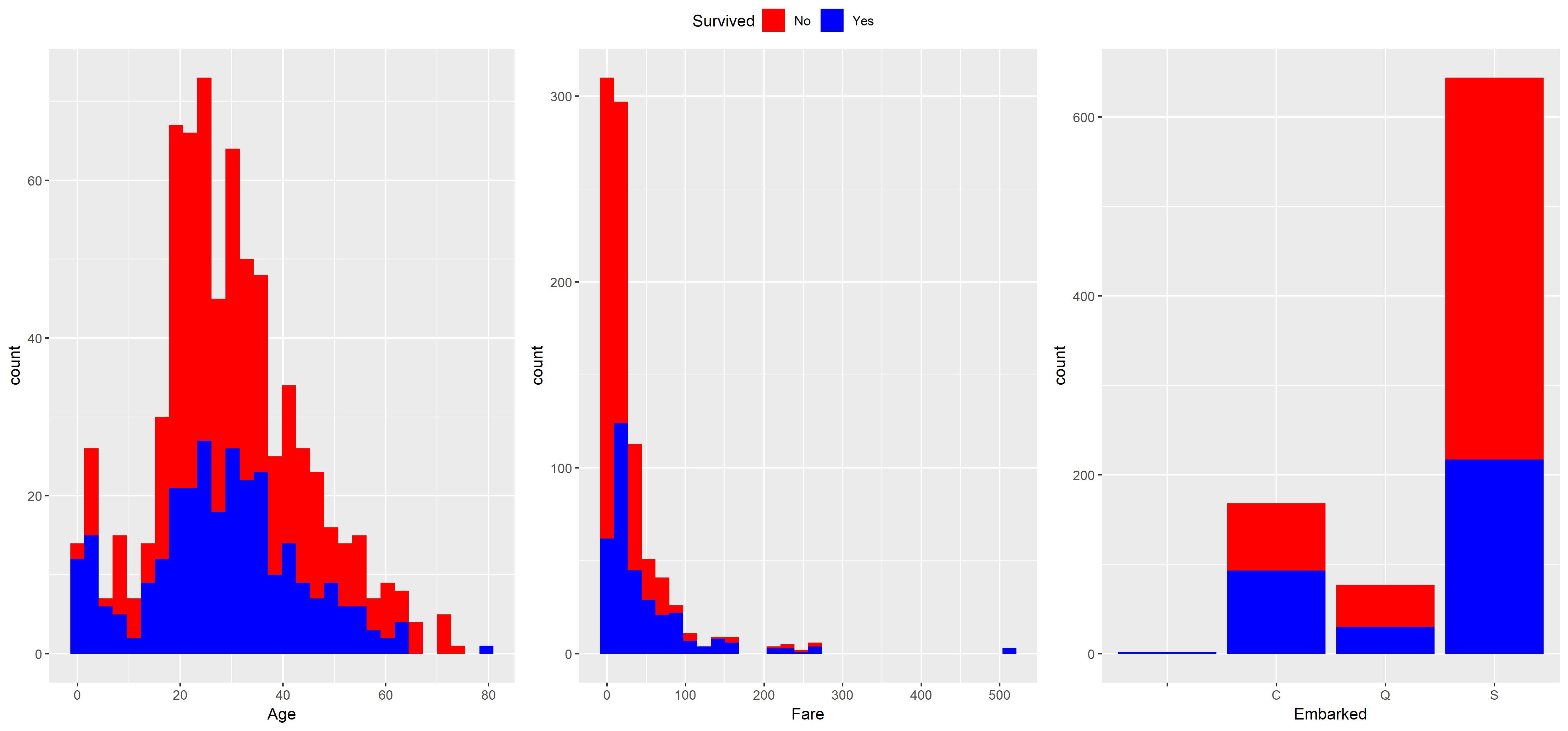
For the Age variable, we can see that younger children are more likely to survive. From around 0 – 10, the survival chances are pretty good.
There are a lot of fares that cost around $10. People who paid this amount had really bad survival chances. It seems like the more expensive the fare, the better the survival chances are.
The third plot shows where people embarked. This plot does not say a lot about survival. We can see, however, that we have some missing values there and most people came on board in “S”, which stands for Southampton.

Investigating The Titles of Passengers for the Titanic Data Set

Next, we do some feature engineering. This means we are deriving new variables that have more explanatory power in predicting who survived and died from already existing variables in the data set. Such a variable is Name for example. In order to do that, it is advantageous to have some basic understanding of regular expressions. When I first looked at other people’s kernels, I had no idea how they got the titles out of the name variable. The code looks pretty complicated and it takes some time to get used to regular expressions.

head(titanic$Name)

## [1] "Braund, Mr. Owen Harris"                            
## [2] "Cumings, Mrs. John Bradley (Florence Briggs Thayer)"
## [3] "Heikkinen, Miss. Laina"                             
## [4] "Futrelle, Mrs. Jacques Heath (Lily May Peel)"       
## [5] "Allen, Mr. William Henry"                           
## [6] "Moran, Mr. James"

When we look at the output of the head function, then we see that every passenger name starts with their last name, followed by a comma, followed by their title with a dot, and then their first names. We are going to extract the title with the gsub() function.

Here is a little working example. In order to extract the title of my name from the string below we are saying that everything before and including the comma should be removed and then everything after and including the dot should be removed as well.

x <- "Schmidt, Mr. Pascal David Fabian"

We do that with the code below. The .*, means that we remove everything before the comma. The comma (,) is a special character and therefore, we need these two backward slashes (\) in front of the comma. Then we have the “or” (|) bar. After that, we need the two backward slashes again because the literal dot after the titles is also a special character. Then we say remove everything after the dot again. So what we are doing is replacing “Schmidt,” with nothing and then ” Pascal David Fabian” with nothing as well. And voila, we are left with the title only.

gsub("(.*\\,|\\..*)", "", x) %>%
  gsub("[[:space:]]", "", .)

## [1] "Mr"

We do that for the entire Name vector, saving the titles in the titles object, and then displaying how many titles there are with the table() function.

titanic$titles <- gsub("(.*\\,|\\..*)", "", titanic$Name) %>%
  gsub("[[:space:]]", "", .)
table(titanic$titles) %>%
  pander::pandoc.table(split.table = Inf)

After that, we are going to do some visualizations. Of course in ggplot2 again!

title_sum <- titanic[1:891, ] %>%
  group_by(titles, Survived) %>%
  summarise(freq = n()) %>%
  ungroup() %>%
  mutate(
    total = sum(freq),
    prop = freq / total
  )

ggplot(title_sum, aes(x = titles, y = prop, group = Survived)) +
  geom_col(aes(fill = Survived), position = "fill") +
  geom_text(aes(label = freq), position = position_fill(vjust = .5), col = "white") +
  scale_fill_manual(
    name = "Survived",
    values = c("red", "blue"),
    labels = c("No", "Yes"),
    breaks = c("0", "1")
  ) +
  theme(
    plot.title = element_text(hjust = 0.5),
    axis.text.x = element_text(angle = -45, hjust = 0)
  )

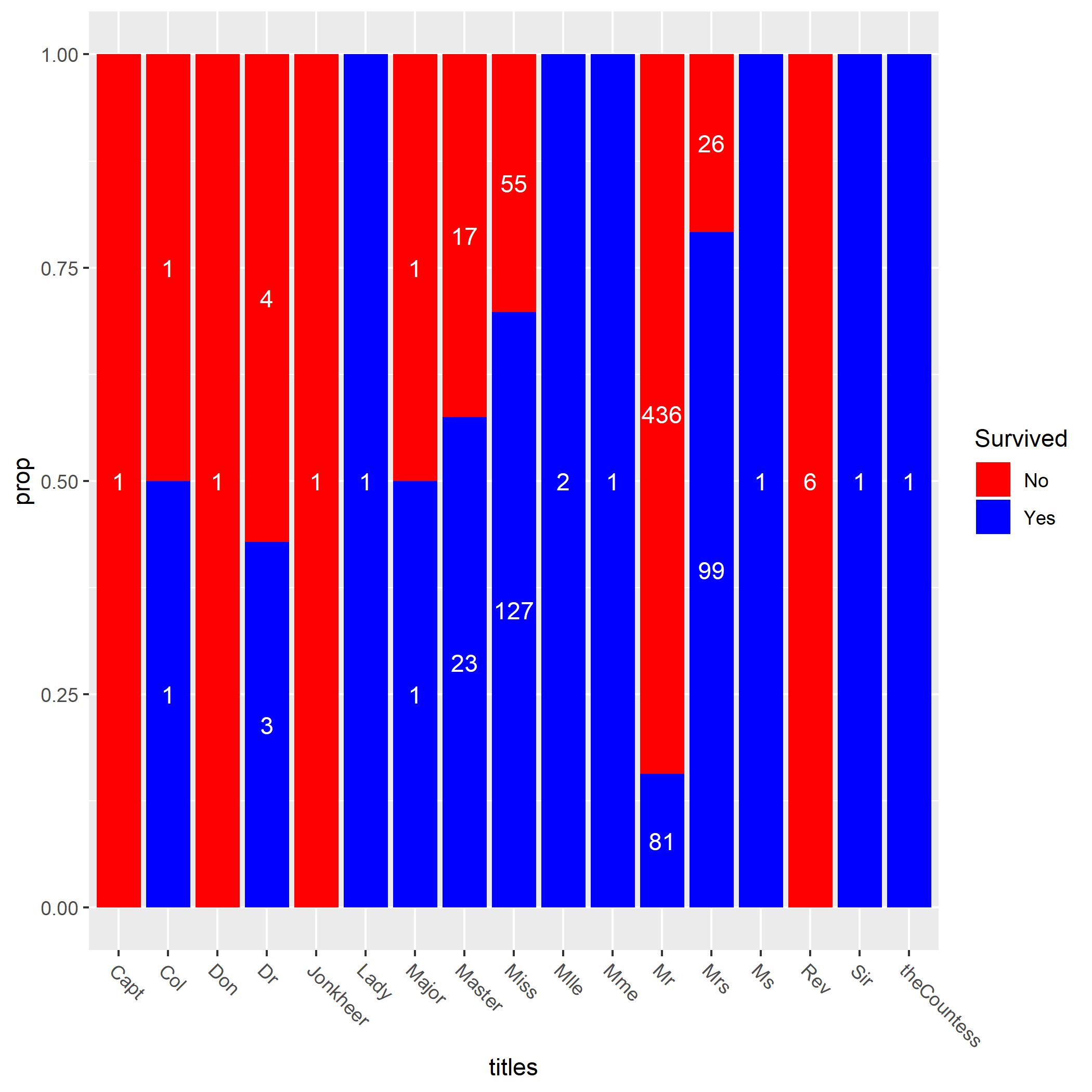
We do some data manipulation with dplyr in order to see the percentage of survived versus dead passengers for each unique title. Then we are plotting. Aouch, a lot of misters died! Wow, that’s actually quite interesting. Mrs and Miss does pretty well. So let’s group some of the titles together. We do that with the code below.

titanic$titles[titanic$titles %in% c("Lady", "theCountess", "Dona", "Jonkheer", "Don", "Sir", "Dr")] <- "Rare Titles"
titanic$titles[titanic$titles %in% c("Ms", "Mme", "Mlle")] <- "Mrs"
titanic$titles[titanic$titles %in% c("Capt", "Col", "Major", "Rev")] <- "Officers"
titanic$titles <- as.factor(titanic$titles)

summary(tableby(Survived ~ titles,
  data = titanic,
  test = FALSE,
  total = FALSE
))

Investigating Cabin Numbers for the Titanic Data Set

A lot of cabin numbers are missing. This is really unfortunate because I think based on the visualization, our final model could have improved from the correct cabin numbers of every single passenger.

titanic$Cabin_letter <- substr(titanic$Cabin, 1, 1)
titanic$Cabin_letter[titanic$Cabin_letter == ""] <- "Unkown"

title_sum <- titanic[1:891, ] %>%
  group_by(Cabin_letter, Survived) %>%
  summarise(freq = n()) %>%
  ungroup() %>%
  mutate(
    total = sum(freq),
    prop = freq / total
  )

ggplot(title_sum, aes(x = Cabin_letter, y = prop, group = Survived)) +
  geom_col(aes(fill = Survived), position = "fill") +
  geom_text(aes(label = freq), position = position_fill(vjust = .5), col = "white") +
  scale_fill_manual(
    name = "Survived",
    values = c("red", "blue"),
    labels = c("No", "Yes"),
    breaks = c("0", "1")
  ) +
  theme(plot.title = element_text(hjust = 0.5)) +
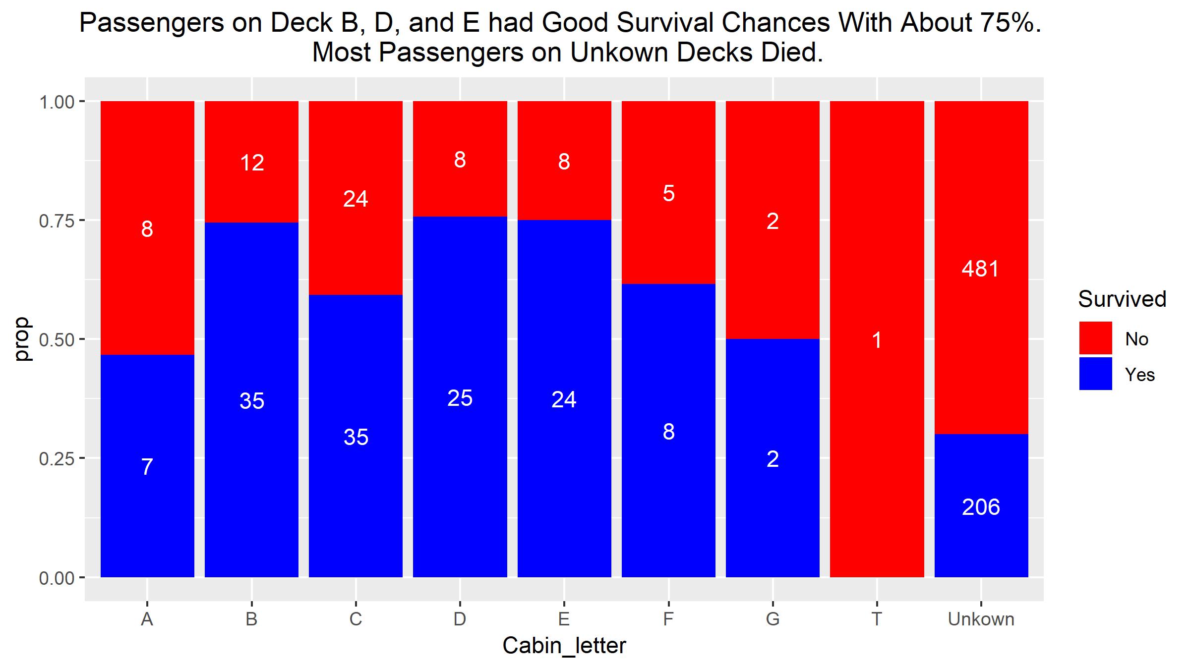
  ggtitle("Passengers on Deck B, D, and E had Good Survival Chances With About 75%. \n Most Passengers on Unkown Decks Died.")

titanic$Cabin_letter <- as.factor(titanic$Cabin_letter)

The cabin numbers are representing on which deck each passenger had their cabin. Survival is pretty good for decks B, D, and E. A lot of passengers from unknown cabin numbers died. Unfortunately, there are too many missing values in the Cabin variable.

Next, we are investigating the family sizes of passengers. SibSp is the number of siblings or spouses on board of the titanic. Parch is the number of parents or children on board the titanic. So we are feature engineering a variable called family_size which will consist of Parch, SibSp and the passenger themself.

Investigating Survival Chances of Families for the Titanic Data Set

titanic$family_size <- titanic$SibSp + titanic$Parch + 1

ggplot(titanic[1:891, ], aes(x = family_size, fill = Survived)) +
  geom_bar() +
  scale_fill_manual(
    name = "Survived",
    values = c("red", "blue"),
    labels = c("No", "Yes"),
    breaks = c("0", "1")
  ) +
  theme(plot.title = element_text(hjust = 0.5)) +
  scale_x_continuous(breaks = seq(1, 11, 1)) +
  ggtitle("Most People Travelled By Themselves. \n Survival is highest for Couples and Parents With 1 and 2 Children. \n For Families With More Than 2 Children Survival Chances are Bad.")

titanic$family_size[titanic$family_size %in% c("5", "6", "7", "8", "9", "10", "11")] <- "Big Family"
titanic$family_size <- as.factor(titanic$family_size)

It seems like survival is highest for couples and parents with 1-3 children. For larger sized families and people traveling alone, survival chances do not seem to be great. Because it seems like larger family sizes do not do well, we are grouping them.

Dealing With Missing Values

Age

missing_row_age <- which(is.na(titanic$Age))

for (i in unique(titanic$titles)) {
  titanic[missing_row_age, "Age"][titanic[missing_row_age, "titles"] == i] <- median(subset(titanic, titles == i)$Age, na.rm = TRUE)
}

First, we identified which rows are missing for the titanic data set. Afterward, we constructed a for loop which imputes every missing age value with the median age of their corresponding title.

Embarked

ggplot(titanic[1:891, ], aes(x = Embarked, fill = Survived)) +
  geom_bar() +
  scale_fill_manual(
    name = "Survived",
    values = c("red", "blue"),
    labels = c("No", "Yes"),
    breaks = c("0", "1")
  ) +
  theme(plot.title = element_text(hjust = 0.5)) +
  ggtitle("Most people got on in Southampton")

titanic$Embarked[titanic$Embarked == ""] <- "S"

The mode of the Embarked variable is Southampton. Therefore, we are substituting the empty string of the two passengers with an S.

Fare

titanic[is.na(titanic$Fare), ] %>%
  select(Age, Fare, Name, Pclass, titles, Embarked) %>%
  pander::pandoc.table(split.table = Inf)
titanic$Fare[is.na(titanic$Fare)] <- median(subset(titanic, Pclass == "3")$Fare, na.rm = TRUE)

In order to impute the one missing value for Fare, we are looking at the median of class 3 fare. Then we are imputing the value.

Model Building

Logistic Regression

model <- glm(Survived ~ Pclass + titles + Fare + family_size + 
                        Parch + SibSp + Embarked + Age + Sex, 
                        family = "binomial", data = titanic[1:891, ])
summary(model)

## 
## Call:
## glm(formula = Survived ~ Pclass + titles + Fare + family_size + 
##     Parch + SibSp + Embarked + Age + Sex, family = "binomial", 
##     data = titanic[1:891, ])
## 
## Deviance Residuals: 
##     Min       1Q   Median       3Q      Max  
## -2.7414  -0.5232  -0.3937   0.5439   2.4226  
## 
## Coefficients:
##                         Estimate Std. Error z value Pr(>|z|)    
## (Intercept)            19.293975 505.551206   0.038 0.969557    
## Pclass2                -1.117691   0.327881  -3.409 0.000652 ***
## Pclass3                -2.068292   0.323743  -6.389 1.67e-10 ***
## titlesMiss            -15.855578 505.551052  -0.031 0.974980    
## titlesMr               -3.557551   0.607915  -5.852 4.86e-09 ***
## titlesMrs             -15.133361 505.551118  -0.030 0.976119    
## titlesOfficers         -3.672651   1.039915  -3.532 0.000413 ***
## titlesRare Titles      -3.508479   0.956992  -3.666 0.000246 ***
## Fare                    0.003935   0.002667   1.475 0.140132    
## family_size2           -0.271993   0.413730  -0.657 0.510914    
## family_size3           -0.123881   0.712942  -0.174 0.862054    
## family_size4            0.092982   1.104497   0.084 0.932909    
## family_sizeBig Family  -2.539844   1.685012  -1.507 0.131730    
## Parch                  -0.026030   0.356470  -0.073 0.941789    
## SibSp                  -0.155702   0.305080  -0.510 0.609796    
## EmbarkedQ               0.017643   0.401863   0.044 0.964982    
## EmbarkedS              -0.304258   0.257984  -1.179 0.238251    
## Age                    -0.024152   0.009699  -2.490 0.012773 *  
## Sexmale               -15.188611 505.550749  -0.030 0.976032    
## ---
## Signif. codes:  0 '***' 0.001 '**' 0.01 '*' 0.05 '.' 0.1 ' ' 1
## 
## (Dispersion parameter for binomial family taken to be 1)
## 
##     Null deviance: 1186.66  on 890  degrees of freedom
## Residual deviance:  711.52  on 872  degrees of freedom
## AIC: 749.52
## 
## Number of Fisher Scoring iterations: 13

As we can see from the output above, there are some highly significant variables. Moreover, some of the titles are statistically significant too. We did a good job of creating the titles variable. Let’s see what prediction accuracy we get for this model.

testing <- predict(model, type = "response", newdata = titanic[892:1309, ])
titanic[892:1309, ]$Survived <- as.numeric(testing >= 0.5)

pred <- data.frame(titanic[892:1309, ][c("PassengerId", "Survived")])
write.csv(pred, file = "Logit.csv", row.names = FALSE)

One thing that is worrisome about our model is the high standard errors for the Sex and titles variables. This means that the precision for the coefficient estimate is not precise. How can we correct that? With the variance inflation factor (VIF). A VIF value of 5 or below is usually regarded as acceptable.

When we check for multicollinearity among the predictors we can see that the VIF value for the Sex variable is very high. This means that there is multicollinearity in our model which is responsible for inflated standard errors. So, how can we deal with that?

car::vif(model)

##                     GVIF Df GVIF^(1/(2*Df))
## Pclass      2.315854e+00  2        1.233610
## titles      1.709214e+07  5        5.287856
## Fare        1.711375e+00  1        1.308195
## family_size 3.044354e+01  4        1.532628
## Parch       8.342044e+00  1        2.888260
## SibSp       9.137712e+00  1        3.022865
## Embarked    1.356503e+00  2        1.079208
## Age         1.874363e+00  1        1.369074
## Sex         6.716106e+06  1     2591.545055

One common solution is to standardize the variables with a high variance inflation factor. If this does not yield success, then throwing them out of the model is another solution. For our model, we are deciding to throw away the Sex variable.

After having done that, you will realize that there is still multicollinearity in our model. The VIF values for Parch, SibSp, and family_size are still high. This is not really a surprise. Remember, we derived the family_size variable from the SibSp and Parch variable. We are deciding to throw away our derived variable family_size and then have another look at the VIF values.

car::vif(model_reduced)

##              GVIF Df GVIF^(1/(2*Df))
## Pclass   2.256789  2        1.225668
## titles   3.047385  5        1.117874
## Fare     1.623189  1        1.274044
## Parch    1.463319  1        1.209677
## SibSp    1.597912  1        1.264085
## Embarked 1.285848  2        1.064872
## Age      1.959045  1        1.399659

Now, that looks much better! No single variable is above 5 anymore. In addition to that, our model output looks much better now.

model_reduced <- glm(Survived ~ Pclass + titles + Fare + Parch + SibSp + 
                              Embarked + Age, family = "binomial", 
                              data = titanic[1:891, ])
summary(model_reduced)

## 
## Call:
## glm(formula = Survived ~ Pclass + titles + Fare + Parch + SibSp + 
##     Embarked + Age, family = "binomial", data = titanic[1:891, 
##     ])
## 
## Deviance Residuals: 
##     Min       1Q   Median       3Q      Max  
## -2.3862  -0.5491  -0.3832   0.5511   2.5761  
## 
## Coefficients:
##                    Estimate Std. Error z value Pr(>|z|)    
## (Intercept)        4.294896   0.631517   6.801 1.04e-11 ***
## Pclass2           -1.088434   0.322700  -3.373 0.000744 ***
## Pclass3           -2.158943   0.318472  -6.779 1.21e-11 ***
## titlesMiss        -0.522737   0.504034  -1.037 0.299686    
## titlesMr          -3.451705   0.547544  -6.304 2.90e-10 ***
## titlesMrs          0.318030   0.570859   0.557 0.577454    
## titlesOfficers    -3.548728   1.005306  -3.530 0.000416 ***
## titlesRare Titles -2.630036   0.827722  -3.177 0.001486 ** 
## Fare               0.003511   0.002642   1.329 0.183827    
## Parch             -0.354448   0.134171  -2.642 0.008248 ** 
## SibSp             -0.556195   0.125424  -4.435 9.23e-06 ***
## EmbarkedQ         -0.131422   0.393675  -0.334 0.738506    
## EmbarkedS         -0.400157   0.249909  -1.601 0.109330    
## Age               -0.027704   0.009509  -2.914 0.003574 ** 
## ---
## Signif. codes:  0 '***' 0.001 '**' 0.01 '*' 0.05 '.' 0.1 ' ' 1
## 
## (Dispersion parameter for binomial family taken to be 1)
## 
##     Null deviance: 1186.66  on 890  degrees of freedom
## Residual deviance:  729.09  on 877  degrees of freedom
## AIC: 757.09
## 
## Number of Fisher Scoring iterations: 5

As we can see, the standard errors of the coefficients are not high anymore and became more precise. Age became more statistically significant as well as Parch and SibSp. Let’s make another submission!

testing <- predict(model_reduced, type = "response", newdata = titanic[892:1309, ])
titanic[892:1309, ]$Survived <- as.numeric(testing >= 0.5)

pred_reduced <- data.frame(titanic[892:1309, ][c("PassengerId", "Survived")])
write.csv(pred_reduced, file = "Logit_reduced.csv", row.names = FALSE)

Wow! Our model has improved by only doing some variable selection.

Random Forest

randomForest_model <- randomForest(Survived ~ Pclass + Age + SibSp + Parch +
  Fare + Embarked + titles +
  family_size + Sex, ntree = 1000,
data = titanic[1:891, ]
)

importance <- importance(randomForest_model)
var_importance <- data.frame(
  variables = row.names(importance),
  importance = round(importance[, "MeanDecreaseGini"], 2)
)


rank_importance <- var_importance %>%
  mutate(rank = paste0("#", dense_rank(desc(importance))))


ggplot(rank_importance, aes(
  x = reorder(variables, importance),
  y = importance, fill = importance
)) +
  geom_bar(stat = "identity") +
  geom_text(aes(x = variables, y = 0.5, label = rank),
    hjust = 0, vjust = 0.55, size = 4, colour = "red"
  ) +
  labs(x = "Variables") +
  coord_flip()

Let’s send in our predictions!

pred <- predict(randomForest_model, titanic[892:1309, ])

randomForest_pred <- data.frame(PassengerID = titanic[892:1309, ]$PassengerId, Survived = pred)
write.csv(randomForest_Pred, file = "randomForest_model.csv", row.names = F)

titanic data set random forest prediction

The random forest model has the same prediction accuracy as the logistic regression model. Why is that?

A random forest model is great in eliminating muticollinearity. In the code above, we specified that we want to build 1000 trees. Each of those trees is only taking a subset of predictors. In the randomForest() function, the model only chooses $\sqrt{p}$ predictors at each split. In short, the random forest model only considers a subset of predictors at each split which is great to eliminate collinearity. This will lead to a reduction in variance as well. In the book “An Introduction to Statistical Learning“, it says:

“We can think of this process (only taking a subset of predictors) as decorrelating the trees, thereby making the average of the resulting trees less variable and hence more reliable.”

When knowing how a random forest works, it is not surprising that it achieves good accuracy even with a highly correlated data set such as the titanic one.

Linear Discriminant Analysis

I already explained the theory behind LDA and also provided a practical example. So, in this blog post, we are only looking at the prediction accuracy. After, we will see if the model will outperform the previous ones.

lda_model <- MASS::lda(Survived ~ Pclass + titles + Fare + family_size + 
                              Parch + SibSp + Embarked + Age + Sex, 
                              data = titanic[1:891, ])

training_data <- predict(lda_model, type = "response", newdata = titanic[892:1309, ])
testing_data <- data.frame(titanic[892:1309, ]$PassengerId, Survived = training_data$class)
write.csv(testing_data, file = "TitanicPredLDA.csv", row.names = FALSE)

Wow, our best prediction so far!

K-Nearest Neighbors

The last algorithm that we are going to evaluate is k-nearest neighbors. The critical part of this algorithm is to select the flexibility of the algorithm. The fewer neighbors, the more flexible the algorithm is and the more neighbors, the more inflexible the algorithm the greater amount of neighbors.

We determine the perfect amount of neighbors for the titanic data set with the caret package and cross-validation.

# turn every categorical variables into 
# numeric ones for standardization
for (i in names(titanic)) {
  if (is.factor(titanic[, i])) {
    titanic[, i] <- as.double(titanic[, i])
  } else if (is.character(titanic[, i])) {
    titanic <- dplyr::select(titanic, -i)
  }
}

titanic$Survived <- as.factor(titanic$Survived)
titanic <- titanic[, -1] # Remove passengerID
titanic_scaled <- scale(titanic[, -1]) # Standardize every variable except for Survived

# 5-fold cross-validation
trControl <- caret::trainControl(
  method = "cv",
  number = 5
)

fit <- caret::train(Survived ~ .,
  method = "knn",
  tuneGrid = expand.grid(k = 1:10),
  trControl = trControl,
  metric = "Accuracy",
  data = titanic[1:891, ]
)

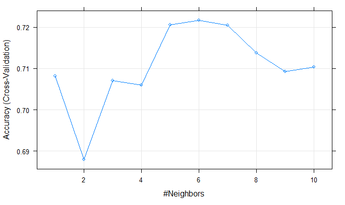
As we can see in the plot above, the best accuracy is achieved by 6 neighbors. Therefore, we will choose k = 6 in our knn algorithm from the class package.

knn_predictions <- class::knn(titanic_scaled[1:891, -1], 
                              titanic_scaled[892:1309, -1], 
                              titanic[1:891, ]$Survived, 
                              k = 6)

knn_predictions
knn_predictions <- ifelse(knn_predictions == 1, 0, 1)

pred <- data.frame(PassengerId = 892:1309, 
                          Survived = knn_predictions)
write.csv(pred, file = "knn.csv", row.names = FALSE)

All of our models give pretty much the same accuracy. However, we have two clear winners for the titanic data set. Our LDA model and our knn model give the best accuracy.

Unfortunately, we have not yet received an accuracy of 80% or higher. In my next blog post, we will though. After some research, I came along the gender model which will boost our accuracy to 82%.

I hope you have enjoyed this blog post about the titanic data set. If you have any questions let me know in the comments below. Thank you.

Tags: data analysis Kaggle machine learning R Titanic

Titanic Data Set – How I increased my score from 79% to 82%