Cross-Validation the Wrong Way and Right Way With Feature Selection
Cross-validation is a popular technique to evaluate true model accuracy. However, cross-validation is not as straight forward as it may seem and can provide false confidence. This means that it is easy to overfit when not done properly. So, how can we avoid doing cross-validation the wrong way?

First, I will be going over one pitfall of cross-validation called data leakage.
What is Data Leakage?
The PC Magazine Encyclopedia defines data leakage as:
The unauthorized transfer of classified information from a computer or datacenter to the outside world.
The classified information in terms of cross-validation is the data in the test set. A computer or data center would be the test set and the outside world the training set.
In other words, data leakage can happen when we are learning from both, the testing and training set. If we do any pre-processing outside the cross-validation algorithm, we will bias our results and most likely overfit our model.
So, consider a scenario where we want to reduce our predictors. We can do that by stepwise selection or for example based on correlations. So we are doing some sort of variable selection and then applying k-fold cross-validation to our data set to estimate the test set error.
The problem arises when using our training and testing data set for variable selection. This results in a biased estimate of our model accuracy. In other words, our k-fold cross-validation accuracy is an overestiamte of the true test set error.
What we are going to cover:
- We will be presenting how to do cross-validation the wrong way and the right way. We will be looking at a real data set (Pima Indians Data Set).
- In order to make the difference between a right cross-validation loop and a wrong cross-validation loop more visible, we will be creating a random data set and compare accuracies. Then, we will be visualizing the difference between the right and wrong cross-validation method.
- What kind of pre-processing is allowed before applying cross-validation? Which procedures lead to overfitting?
Let’s get started!
Doing Cross-Validation the Wrong Way (Pima Indians Data Set)
Here is an example of the Pima Indians data set. There are 9 variables in the data set. One response variable (being diabetic or not) and 8 explanatory variables.
After some pre-processing of the data, we are left with 392 rows. Because we do not have many samples (only 392) we will be doing 5-fold cross-validation instead of 10-fold cross-validation.
We will be getting some help from the caret package.
What Happens in our Cross-Validation Loop?
In the section below, there is a short explanation of our cross-validation loop:
- First, we are creating 5 folds with the
caretpackage. Each fold has roughly the same amount of data. - Then we are creating a testing and a training data set. The testing data set consists of 1 out of 5 folds and the training set consists of 4 out of 5 folds.
- After that, we are doing some variable selection based on the highest correlation. This is the step where the mistake happens. In this step, we are combining the test and training sets. Based on the entire data set, we are finding the highest correlated variables with our response variable.
This is wrong!!!
Instead, we should only use the training data set to find the variables with the highest correlations. Hence, not touching the test set. Let’s continue in our loop.
- In the next step, we are picking the two variables with the highest correlation.
- Then we are plugging these two variables in our logistic regression model.
- After that, we are predicting our outcomes and rounding the predicted probability scores to 0 or 1.
- Then, we are putting the predicted and actual outcomes in a data frame, converting these variables to factors, and using the
confusionMatrixfunction to evaluate our model accuracy.
In between, I inserted a print statement so you can see which variables we are selecting in each fold.
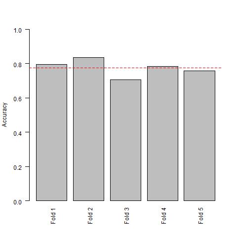
Because we are using the entire data set to select features, we are getting the same features in each loop. Namely Glucose and Age. This is exactly how you do cross-validation the wrong way.
set.seed(100)
diabetes <- read.csv(here::here("docs", "diabetes.csv"))
diabetes[, 2:6][diabetes[, 2:6] == 0] <- NA
diab <- na.omit(diabetes)
diab$ID <- c(1:(nrow(diab)))

confusion_matrices <- list()
accuracy <- c()
for (i in c(1:5)) {
  # creating 5 random folds from the cancer data set
  folds <- caret::createFolds(diab$Outcome, k = 5)

  # splitting the data into training and testing
  test <- diab[diab$ID %in% folds[[i]], ]
  train <- diab[diab$ID %in% unlist(folds[-i]), ]

  # doing feature selection by choosing the 2 "best" predictors
  # based on the highest correlation coefficients
  data.frame(correlation = cor(rbind(train, test))[, "Outcome"]) %>%
    tibble::rownames_to_column(., var = "predictor") %>%
    dplyr::arrange(., desc(correlation)) -> df_correlation

  # pick the two columns with the highest correlation
  # and the response variable (diagnosis)
  df_highest_correlation <- c(df_correlation[c(1, 2, 3), 1])
  print(df_highest_correlation)

  # building a logistic regression model based on the 2 predictors
  # with the highest correlation from the previous step
  glm_model <- glm(as.factor(Outcome) ~ ., family = binomial, data = train[, df_highest_correlation])

  # making predictions
  predictions <- predict(glm_model, newdata = test[, df_highest_correlation], type = "response")

  # rounding predictions
  predictions_rounded <- as.numeric(predictions >= 0.5)


  predictions_df <- data.frame(cbind(test$Outcome, predictions_rounded))
  predictions_list <- lapply(predictions_df, as.factor)
  confusion_matrices[[i]] <- caret::confusionMatrix(predictions_list[[2]], predictions_list[[1]])
  accuracy[[i]] <- confusion_matrices[[i]]$overall["Accuracy"]
}

[1] “Outcome” “Glucose” “Age”
[1] “Outcome” “Glucose” “Age”
[1] “Outcome” “Glucose” “Age”
[1] “Outcome” “Glucose” “Age”
[1] “Outcome” “Glucose” “Age”
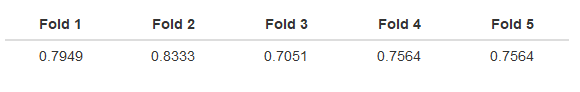
names(accuracy) <- c("Fold 1", "Fold 2", "Fold 3", "Fold 4", "Fold 5")
accuracy %>%
  pander::pandoc.table()

mean(accuracy)
[1] 0.774359

names(accuracy) <- c("Fold 1", "Fold 2", "Fold 3", "Fold 4", "Fold 5")
barplot(
  accuracy,
  ylim = c(0, 1), las = 2,
  ylab = "Accuracy"
)

abline(h = mean(accuracy), col = "red", lty = 2)
Doing Cross-Validation the Right Way (Pima Indians Data Set)
Let’s see how to do cross-validation the right way.
The code below is basically the same as the above one with one little exception.
In step three, we are only using the training data to do the feature selection. This ensures, that there is no data leakage and we are not using information that is in the test set to help with feature selection.
After we are done, we can see that during our fourth loop, the algorithm chooses Glucose and Insulin as being the “best” predictors (based on the correlation coefficient). However, for all other loops, the algorithm still chooses Glucose and Age as our “best” predictors.
set.seed(100)
diabetes <- read.csv(here::here("docs", "diabetes.csv"))
diabetes[, 2:6][diabetes[, 2:6] == 0] <- NA
diab <- na.omit(diabetes)
diab$ID <- c(1:(nrow(diab)))

confusion_matrices <- list()
accuracy <- c()
for (i in c(1:5)) {
  # creating 5 random folds from the cancer data set
  folds <- caret::createFolds(diab$Outcome, k = 5)

  # splitting the data into training and testing
  test <- diab[diab$ID %in% folds[[i]], ]
  train <- diab[diab$ID %in% unlist(folds[-i]), ]

  # doing feature selection by choosing the 2 "best" predictors
  # based on the highest correlation coefficients
  data.frame(correlation = cor(train)[, "Outcome"]) %>%
    tibble::rownames_to_column(., var = "predictor") %>%
    dplyr::arrange(., desc(correlation)) -> df_correlation

  # pick the two columns with the highest correlation
  # and the response variable (diagnosis)
  df_highest_correlation <- c(df_correlation[c(1, 2, 3), 1])
  print(df_highest_correlation)

  # building a logistic regression model based on the 2 predictors
  # with the highest correlation from the previous step
  glm_model <- glm(as.factor(Outcome) ~ ., family = binomial, data = train[, df_highest_correlation])

  # making predictions
  predictions <- predict(glm_model, newdata = test[, df_highest_correlation], type = "response")

  # rounding predictions
  predictions_rounded <- as.numeric(predictions >= 0.5)


  df <- data.frame(cbind(test$Outcome, predictions_rounded))
  df <- lapply(df, as.factor)
  confusion_matrices[[i]] <- caret::confusionMatrix(df[[2]], df[[1]])
  accuracy[[i]] <- confusion_matrices[[i]]$overall["Accuracy"]
}

[1] “Outcome” “Glucose” “Age”
[1] “Outcome” “Glucose” “Age”
[1] “Outcome” “Glucose” “Age”
[1] “Outcome” “Glucose” “Insulin”
[1] “Outcome” “Glucose” “Age”
names(accuracy) <- c("Fold 1", "Fold 2", "Fold 3", "Fold 4", "Fold 5")
accuracy %>%
  pander::pandoc.table()
mean(accuracy)
[1] 0.7692308

names(accuracy) <- c("Fold 1", "Fold 2", "Fold 3", "Fold 4", "Fold 5")
barplot(
  accuracy,
  ylim = c(0, 1), las = 2,
  ylab = "Accuracy"
)

abline(h = mean(accuracy), col = "red", lty = 2)
So the questions we have to answer are now: “How are we supposed to continue?” and “Is the error from the right cross-validation loop our test set error?”
The next step is to choose features that have the maximum number of votes. In this case, it is Glucose and Age. Now, we have to do another round of cross-validation on only these sets of features.
Luckily in this example, doing feature selection and cross-validation the wrong way and the right way, gave us identical features. So, our cross-validation test set error in the first code block would not be biased.
However, it could have been that our second code block, where we did cross-validation the right way, had given us completely different features. Then, the test set error in the first code block would have been extremely biased.
Getting extremely biased results when doing cross-validation the wrong way usually happens with wider data sets. So, with data sets that have hundreds of predictors and just a small amount of samples. (You will see that later on our simulated data).
So, as we said, we are doing cross-validation again with the majority of features selected in code block 2 (Glucose and Age). This is because cross-validation should only be used to measure how a SINGLE model performs on a given test set. If we are comparing models that have Glucose and Age with models that have Glucose and Insulin as predictors, then we are not comparing the performance correctly.
Cross-Validation With the Caret Package
The following code does everything for us. So, we are not ending up with a lot of lines of code.
train_control <- trainControl(method = "cv", number = 5)
model_glm <- train(as.factor(Outcome) ~ Glucose + Age,
                   trControl = train_control,
                   method = "glm",
                   data = diab)
predictions_glm <- predict(model_glm, diab)
confusionMatrix(predictions_glm, as.factor(diab$Outcome))

## Confusion Matrix and Statistics
##
##           Reference
## Prediction   0   1
##          0 233  56
##          1  29  74
##
##                Accuracy : 0.7832
##                  95% CI : (0.739, 0.823)
##     No Information Rate : 0.6684
##     P-Value [Acc > NIR] : 3.836e-07
##
##                   Kappa : 0.4839
##  Mcnemar's Test P-Value : 0.004801
##
##             Sensitivity : 0.8893
##             Specificity : 0.5692
##          Pos Pred Value : 0.8062
##          Neg Pred Value : 0.7184
##              Prevalence : 0.6684
##          Detection Rate : 0.5944
##    Detection Prevalence : 0.7372
##       Balanced Accuracy : 0.7293
##
##        'Positive' Class : 0
##
The accuracy here is different from the accuracy we got in our first code block even though we used the same features. This is because of the caret functions are using different splits for the data.
Doing Cross-Validation the Right Way With a Simulated Data Set
Now let’s consider an example where the accuracy between doing cross-validation the wrong way and the right way is more evident.
First, we are creating 100 samples, 5000 predictors, and 1 response variable randomly. Hence, we have a very wide data set. We know exactly how the explanatory variables are related to the response variable. The answer is that there is no relationship. All the correlation that will be created occurs by chance.
So theoretically, the accuracy of the test set should be 50%. In other words, it shouldn’t be better than guessing.
Let’s see what happens when we perform cross-validation the right way.
set.seed(205)
n <- 100
p <- 5000
X <- as.data.frame(matrix(rnorm(n * p), n))
Y <- as.numeric(runif(50) < 0.5)
X$Y <- Y
X$ID <- c(1:(nrow(X)))


confusion_matrices <- list()
accuracy <- c()
for (i in c(1:5)) {
  # creating 5 random folds from the cancer data set
  folds <- caret::createFolds(X$Y, k = 5)

  # splitting the data into training and testing
  test <- X[X$ID %in% folds[[i]], ]
  train <- X[X$ID %in% unlist(folds[-i]), ]

  # doing feature selection by choosing the 2 "best" predictors
  # based on the highest correlation coefficients
  data.frame(correlation = abs(cor(train)[, "Y"])) %>%
    tibble::rownames_to_column(., var = "predictor") %>%
    dplyr::arrange(., desc(correlation)) -> df_correlation

  # pick the two columns with the highest correlation
  # and the response variable (diagnosis)
  df_highest_correlation <- c(df_correlation[c(1, 2, 3), 1])
  print(df_highest_correlation)

  # building a logistic regression model based on the 2 predictors
  # with the highest correlation from the previous step
  glm_model <- glm(as.factor(Y) ~ ., family = binomial, data = train[, df_highest_correlation])

  # making predictions
  predictions <- predict(glm_model, newdata = test[, df_highest_correlation], type = "response")

  # rounding predictions
  predictions_rounded <- as.numeric(predictions >= 0.5)

  # Evaluating model accuracy
  predictions_df <- data.frame(cbind(test$Y, predictions_rounded))
  predictions_list <- lapply(predictions_df, as.factor)
  confusion_matrices[[i]] <- caret::confusionMatrix(predictions_list[[2]], predictions_list[[1]])
  accuracy[[i]] <- confusion_matrices[[i]]$overall["Accuracy"]
}

[1] “Y” “V3891” “V3987”
[1] “Y” “V2453” “V1248”
[1] “Y” “V4549” “V3891”
[1] “Y” “V2807” “V1183”
[1] “Y” “V3915” “V68”
mean(accuracy)
[1] 0.48
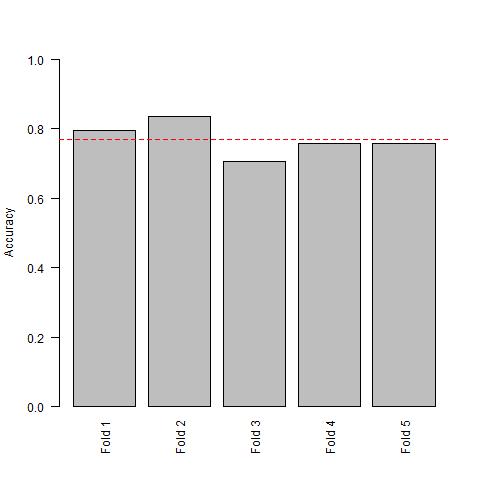
names(accuracy) <- c("Fold 1", "Fold 2", "Fold 3", "Fold 4", "Fold 5")
accuracy %>%
pander::pandoc.table()
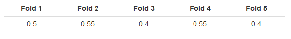
mean(accuracy)
[1] 0.48

names(accuracy) <- c("Fold 1", "Fold 2", "Fold 3", "Fold 4", "Fold 5")
barplot(
  accuracy,
  ylim = c(0, 1), las = 2,
  ylab = "Accuracy"
)

abline(h = mean(accuracy), col = "red", lty = 2)
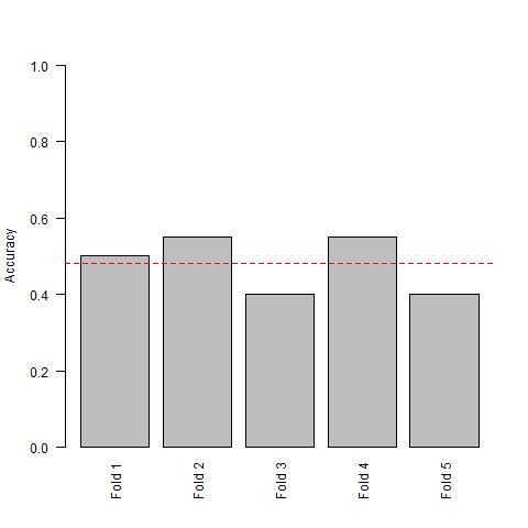
As expected, we are getting around 48% accuracy which is no better than guessing.
Moreover, we are noticing that our predictors are always different and changing. This indicates that there is no consistency across our data set. Choosing predictors is random and we should conclude that we can’t build a predictive model based on the data set.
What would have happened, however, if we had included the test data? So, if we had done cross-validation the wrong way?
Doing Cross-Validation the Wrong Way With a Simulated Data Set
Let’s find out. Below is the code where we do cross-validation the wrong way. Again, the only difference is that we are including the test data set when choosing the predictors with the highest correlation coefficient.
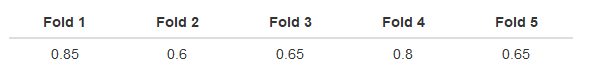
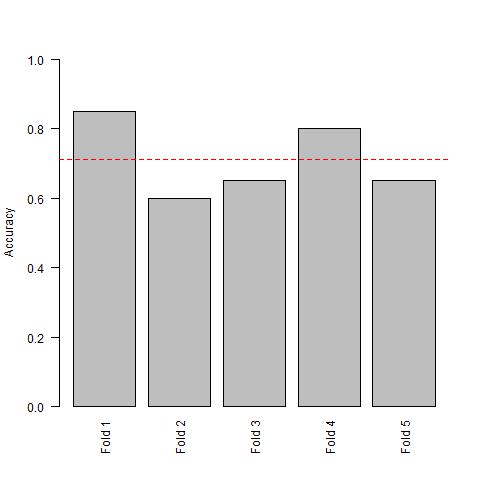
It is no surprise, that we see the same two predictors for each iteration. V4827 and V1293 pop up every time.
If we had no idea that we have applied cross-validation the wrong way, choosing V4827 and V1293 seems like a reasonable choice to make. Moreover, these predictors give us 70% accuracy. This is very good depending on the problem at hand.
Thankfully, we know that there is no relationship between predictors and response variables. Therefore, a 70% accuracy is a gross overestimation of the test set accuracy.
set.seed(123)
n <- 100
p <- 5000
X <- as.data.frame(matrix(rnorm(n * p), n))
Y <- as.numeric(runif(50) < 0.5)
X$Y <- Y
X$ID <- c(1:(nrow(X)))


confusion_matrices <- list()
accuracy <- c()
for (i in c(1:5)) {
  # creating 5 random folds from the cancer data set
  folds <- caret::createFolds(X$Y, k = 5)

  # splitting the data into training and testing
  test <- X[X$ID %in% folds[[i]], ]
  train <- X[X$ID %in% unlist(folds[-i]), ]

  # doing feature selection by choosing the 2 "best" predictors
  # based on the highest correlation coefficients
  data.frame(correlation = abs(cor(rbind(train, test)))[, "Y"]) %>%
    tibble::rownames_to_column(., var = "predictor") %>%
    dplyr::arrange(., desc(correlation)) -> df_correlation

  # pick the two columns with the highest correlation
  # and the response variable (diagnosis)
  df_highest_correlation <- c(df_correlation[c(1, 2, 3), 1])
  print(df_highest_correlation)

  # building a logistic regression model based on the 2 predictors
  # with the highest correlation from the previous step
  glm_model <- glm(as.factor(Y) ~ ., family = binomial, data = train[, df_highest_correlation])

  # making predictions
  predictions <- predict(glm_model, newdata = test[, df_highest_correlation], type = "response")

  # rounding predictions
  predictions_rounded <- as.numeric(predictions >= 0.5)


  predictions_df <- data.frame(cbind(test$Y, predictions_rounded))
  predictions_list <- lapply(predictions_df, as.factor)
  confusion_matrices[[i]] <- caret::confusionMatrix(predictions_list[[2]], predictions_list[[1]])
  accuracy[[i]] <- confusion_matrices[[i]]$overall["Accuracy"]
}
[1] “Y” “V4827” “V1293”
[1] “Y” “V4827” “V1293”
[1] “Y” “V4827” “V1293”
[1] “Y” “V4827” “V1293”
[1] “Y” “V4827” “V1293”
mean(accuracy)
[1] 0.71

names(accuracy) <- c("Fold 1", "Fold 2", "Fold 3", "Fold 4", "Fold 5")
accuracy %>%
  pander::pandoc.table()
names(accuracy) <- c("Fold 1", "Fold 2", "Fold 3", "Fold 4", "Fold 5")
barplot(
  accuracy,
  ylim = c(0, 1), las = 2,
  ylab = "Accuracy"
)

abline(h = mean(accuracy), col = "red", lty = 2)
Let’s compare our results to the caret package.
Cross-Validation With the Caret Package
train_control <- trainControl(method = "cv", number = 5)
model_glm <- train(as.factor(Y) ~ V4827 + V1293, trControl = train_control, method = "glm", data = X)
predictions_glm <- predict(model_glm, X)
confusionMatrix(predictions_glm, as.factor(X$Y))
## Confusion Matrix and Statistics
##
##           Reference
## Prediction  0  1
##          0 42 17
##          1 14 27
##
##                Accuracy : 0.69
##                  95% CI : (0.5897, 0.7787)
##     No Information Rate : 0.56
##     P-Value [Acc > NIR] : 0.005346
##
##                   Kappa : 0.3663
##  Mcnemar's Test P-Value : 0.719438
##
##             Sensitivity : 0.7500
##             Specificity : 0.6136
##          Pos Pred Value : 0.7119
##          Neg Pred Value : 0.6585
##              Prevalence : 0.5600
##          Detection Rate : 0.4200
##    Detection Prevalence : 0.5900
##       Balanced Accuracy : 0.6818
##
##        'Positive' Class : 0
##
And as expected, the caret package gives us a similar result to our loop. A 69% accuracy is also a great overestimation of the real test set accuracy, which we know is 50%.
In conclusion, cross-validation seems like a very straight forward concept. However, in practice, it is not as easy and we do have to follow certain practices to not overfit a model.
So far, we have talked a lot about how to choose features correctly using cross-validation. However, it is also worth noting what we can do before doing cross-validation.
So what kind of pre-processing is allowed vs. what do we have to include inside the cross-validation loop?
Pre-processing Inside the Cross-Validation Loop Vs. Outside the Loop
Everything is allowed that operates on each sample independently. Therefore, methods like smoothing or normalization are okay. This is because it only works on one sample at a time and doesn’t affect other samples.
Other techniques like centering is a problem because we are subtracting the mean of the entire column from every single observation in the column. Therefore, centering has to be done in the cross-validation loop. Same procedure as with feature selection.
If you enjoyed this blog post, you might also like the post where I am talking about the bias-variance trade-off in machine learning.
If you have any questions or suggestions for improvements, please let me know in the comments below.
Other Recourses
You can find out more about what you can do before cross-validation and what you have to put inside the loop here.
When you want to find out more about the topic then this is a great post about a Kaggle competition, cross-validation, and overfitting the public leaderboard.
Other great resources that show code examples of how to do cross-validation the wrong and right way can be found here and here.
Similar Topics:
Comments (7)
Thanks for this – I enjoyed reading it! But I don’t understand why normalization can be done before CV while centering not. Can you plz explain more details?
Thank you, I am glad you enjoyed the read.
So, take for example the gapminder data set and consider the code below.
ggplot(gapminder, aes(x = log(gdpPercap), y = lifeExp, col = continent)) +

  geom_point()
gapminder %>%
lm(lifeExp ~ gdpPercap, data = .) %>%
summary()
ggplot(gapminder, aes(x = log(gdpPercap), y = lifeExp, col = continent)) +
geom_point()
gapminder %>%
lm(lifeExp ~ log(gdpPercap), data = .) %>%
summary()
Here, we did a log transformation to normalize the data. Each log transformation only operated on a single row and did not depend on other rows. However, when we do scale the data set, then we take into account the mean for example. Therefore, we are taking into account multiple rows.
Hence, when we do cross-validation, we have leave out the fold we are testing on otherwise we would leak information. Therefore, we have to do it inside the cross validation loop.
I just noticed that one of the links was pointing to a wrong address. I updated the link above. Check it out for slightly more detail if you are still confused. Link
There are other normalization techniques where you do take into account other rows. Then you should do the normalization inside the cross validation loop.
Let me know if you have any more questions.
Other different suggestion about normalization(I voted that) is here.
https://stats.stackexchange.com/questions/77350/perform-feature-normalization-before-or-within-model-validation
Thank you so much. Very detailed explanation.
However, I am wondering about the steps after we conduct the cross-validation the right way. You said we should pick predictors that most appear in all the folds and do the cross-validation again. Is it biased too? Is it the same as you cherry-pick meaningful predictors over the entire dataset and do a CV?
I have exactly the same concern because with that we are using the same data during 2nd cross-validation that we used previously during feature selection?
Thank you for this post. It was really easy to understand and it is a very interesting topic I think.