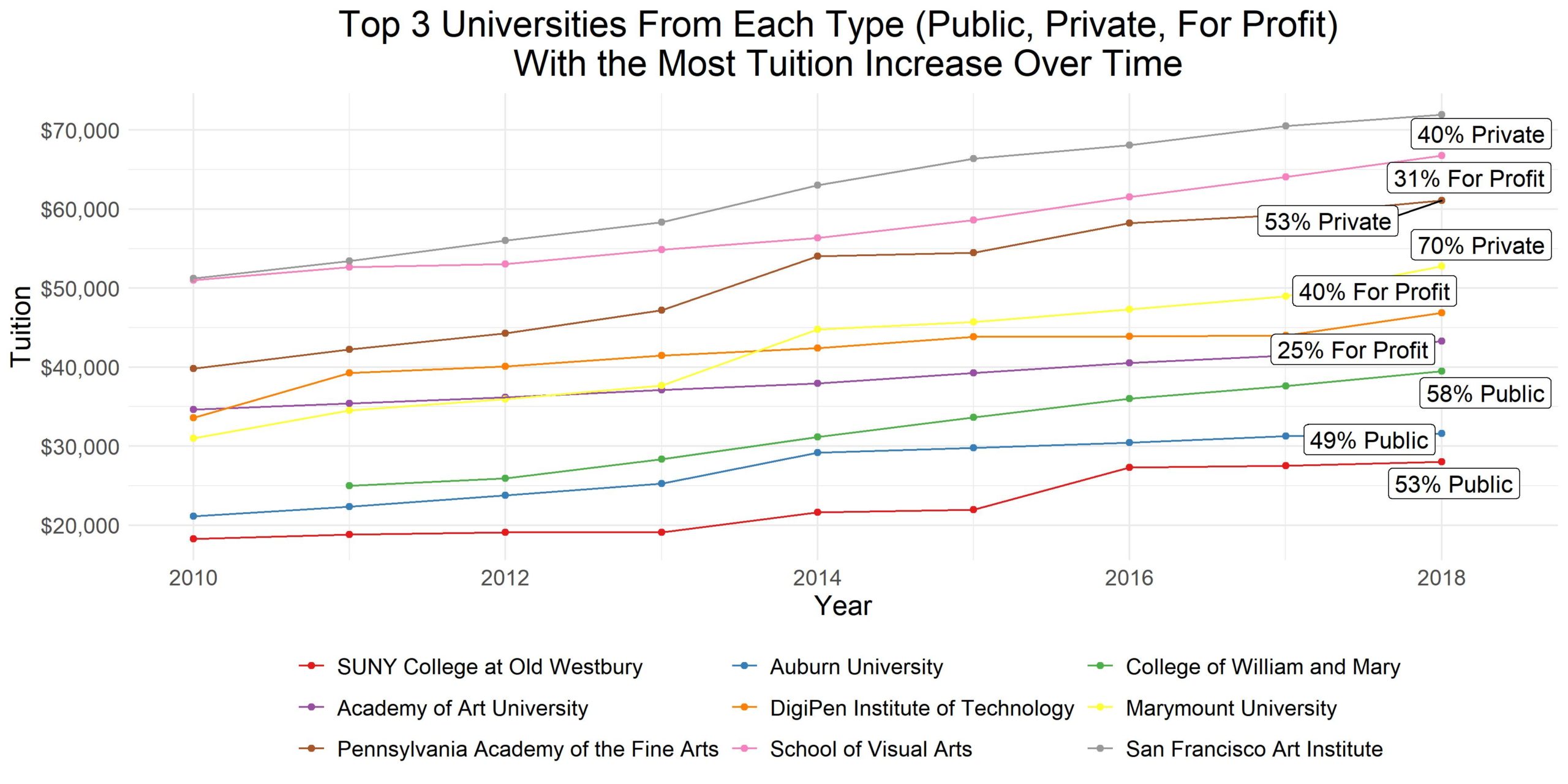
#TidyTuesday – Which Univeristies Have Had the Most Increase in Tuition Costs?
In this blog post, I will be going over my first tidytuesday data set. This data set is about universities in the United States and their tuition. In total, there are three different data sets and they can be explored from many different angles. I decided to look at universities how the tuition cost of universities has been developed over the years.
Hence, the question that I want to answer is:
What universities have had the most increase in tuition costs over the years?
Future students might consider going to the universities listed below when deciding which college to attend.
The data sets can be found here and the code is available on my GitHub.
library(tidyverse)
library(tidytuesdayR)
library(ggrepel)
We need the libraries above. You can get the data with the tidytuesdayR package or you can load in the data with the code below.
tuition_cost <- readr::read_csv('https://raw.githubusercontent.com/rfordatascience/tidytuesday/master/data/2020/2020-03-10/tuition_cost.csv') %>%
  dplyr::select(name, type, degree_length, in_state_tuition)
tuition_income <- readr::read_csv('https://raw.githubusercontent.com/rfordatascience/tidytuesday/master/data/2020/2020-03-10/tuition_income.csv')
Tidytuesday Data Manipulation on Tuition Costs
tuition_income %>%
  dplyr::select(-c(net_cost, income_lvl)) %>%
  dplyr::distinct()

## # A tibble: 44,950 x 5
##    name                              state total_price  year campus
##    <chr>                             <chr>       <dbl> <dbl> <chr>
##  1 Piedmont International University NC          20174  2016 On Campus
##  2 Piedmont International University NC          20514  2017 On Campus
##  3 Piedmont International University NC          20829  2018 On Campus
##  4 Piedmont International University NC          23000  2016 Off Campus
##  5 Piedmont International University NC          26430  2017 Off Campus
##  6 Piedmont International University NC          26870  2018 Off Campus
##  7 Kaplan University-Milwaukee       WI          22413  2017 Off Campus
##  8 Kaplan University-Milwaukee       WI          22492  2018 Off Campus
##  9 Kaplan University-Indianapolis    IN          22413  2017 Off Campus
## 10 Kaplan University-Indianapolis    IN          22492  2018 Off Campus
## # ... with 44,940 more rows
This is how the data looks like. In order to have only distinct years for universities, we will group by year and universities and then use total_price to calculate the average total tuition cost.
tuition_income %>%
  dplyr::group_by(name, year) %>%
  dplyr::summarise(avg_per_year = mean(total_price, na.rm = TRUE)) %>%
  dplyr::ungroup()

## # A tibble: 30,066 x 3
##    name                          year avg_per_year
##    <chr>                        <dbl>        <dbl>
##  1 Aaniiih Nakoda College        2010        17030
##  2 Aaniiih Nakoda College        2011        17030
##  3 Aaniiih Nakoda College        2012        17030
##  4 Aaniiih Nakoda College        2013        17030
##  5 Aaniiih Nakoda College        2014        17030
##  6 Aaniiih Nakoda College        2015        17030
##  7 Aaniiih Nakoda College        2016        17030
##  8 Aaniiih Nakoda College        2017        17030
##  9 Aaniiih Nakoda College        2018        17030
## 10 Abilene Christian University  2011        38250
## # ... with 30,056 more rows
Now, we will be calculating the difference in price from year to year and also count the number of years that are available for each university. Then, we will be filtering out universities that have a negative number in the difference column. We do that because we are only interested in universities that have been increasing tuition costs from year to year.
tuition_income %>%
  dplyr::group_by(name) %>%

  # get difference from year to year for every university
  dplyr::mutate(count = dplyr::n(),
                difference = c(NA, diff(avg_per_year))) %>%

  # filter out universities where tuition was not increasing over time
  dplyr::filter(difference >= 0 | is.na(difference))

## # A tibble: 25,989 x 5
## # Groups:   name [3,664]
##    name                          year avg_per_year count difference
##    <chr>                        <dbl>        <dbl> <int>      <dbl>
##  1 Aaniiih Nakoda College        2010        17030     9         NA
##  2 Aaniiih Nakoda College        2011        17030     9          0
##  3 Aaniiih Nakoda College        2012        17030     9          0
##  4 Aaniiih Nakoda College        2013        17030     9          0
##  5 Aaniiih Nakoda College        2014        17030     9          0
##  6 Aaniiih Nakoda College        2015        17030     9          0
##  7 Aaniiih Nakoda College        2016        17030     9          0
##  8 Aaniiih Nakoda College        2017        17030     9          0
##  9 Aaniiih Nakoda College        2018        17030     9          0
## 10 Abilene Christian University  2011        38250     8         NA
## # ... with 25,979 more rows
Next, we will be creating another count column. The reason for this is that we then compare the two count columns. Whenever the numbers are not equal, we know that this particular university has not had increasing tuition from year to year because we filtered out the negative values earlier. Hence, we throw away universities that have not had increasing tuition.
Afterward, we will be calculating the variance of the price column to see the greatest variation in tuition costs.
Then, we will be joining the data set with the tuition_cost data set to get column names such as type and degree_length. We will also be filtering for 4-year programs.
tuition_income %>%
  # after filtering out universities count again
  dplyr::mutate(count_2 = dplyr::n()) %>%

  # compare counts to first ones and filter out universities
  # that have not had increasing tuition for every single year
  dplyr::filter(count == count_2) %>%

  # calculate variance
  dplyr::mutate(variance = var(avg_per_year, na.rm = TRUE)) %>%

  # only consider universities that hace at least for years of data
  dplyr::filter(count_2 >= 4) %>%
  dplyr::ungroup() %>%
  dplyr::inner_join(tuition_cost %>%
                      dplyr::select(type, name, degree_length), by = "name") %>%

  # only consider universities with 4 years of length
  dplyr::filter(degree_length == "4 Year")

## # A tibble: 6,289 x 9
##    name   year avg_per_year count difference count_2 variance type
##    <chr> <dbl>        <dbl> <int>      <dbl>   <int>    <dbl> <chr>
##  1 Abil~  2011        38250     8         NA       8   1.59e7 Priv~
##  2 Abil~  2012        39900     8       1650       8   1.59e7 Priv~
##  3 Abil~  2013        41800     8       1900       8   1.59e7 Priv~
##  4 Abil~  2014        43100     8       1300       8   1.59e7 Priv~
##  5 Abil~  2015        44740     8       1640       8   1.59e7 Priv~
##  6 Abil~  2016        45980     8       1240       8   1.59e7 Priv~
##  7 Abil~  2017        48300     8       2320       8   1.59e7 Priv~
##  8 Abil~  2018        49722     8       1422       8   1.59e7 Priv~
##  9 Acad~  2010        34648     9         NA       9   8.59e6 For ~
## 10 Acad~  2011        35415     9        767       9   8.59e6 For ~
## # ... with 6,279 more rows, and 1 more variable: degree_length <chr>
Next, we will be splitting our data frame by type (private, for profit, public) into three different data frames. Then we sort each data frame by variance. From these three data frames, we want to grab the first three universities. This is a bit tricky because we do not know the length of the first three universities. This is because some have data with more years than others.
To solve this problem, I used the curly brackets ({}) so suppress magrittr’s pipe behavior and extracted the first three unique names from the name column. I then used str_detect() to filter for these university names.
Afterward, we will be calculating the percentage change from the first year to the last year. Then, we bind the three data frames together again.
tuition_income %>%
  dplyr::group_split(type) %>%
  purrr::map(~ dplyr::arrange(., desc(variance))) %>%

  # only get thetop 3 universities for every type
  purrr::map(~ dplyr::filter(., stringr::str_detect(name, { unique(.$name)[1:3] } %>%
                                                      paste0(collapse = "|")))) %>%
  purrr::map(~ dplyr::group_by(., name)) %>%

  # calculate percentage change from first year to last year
  purrr::map(~ dplyr::mutate(., change_in_price = (dplyr::last(avg_per_year) - avg_per_year[1]) / avg_per_year[1])) %>%
  base::do.call(rbind, .) %>%
  dplyr::ungroup() %>%
  dplyr::filter(name != "Loyola Marymount University") %>%
  dplyr::mutate(name = forcats::fct_reorder(name, avg_per_year),
                date = lubridate::ymd(year, truncated = 2L))

## # A tibble: 80 x 11
##    name   year avg_per_year count difference count_2 variance type
##    <fct> <dbl>        <dbl> <int>      <dbl>   <int>    <dbl> <chr>
##  1 Scho~  2010        50990     9         NA       9   3.00e7 For ~
##  2 Scho~  2011        52650     9       1660       9   3.00e7 For ~
##  3 Scho~  2012        53043     9        393       9   3.00e7 For ~
##  4 Scho~  2013        54883     9       1840       9   3.00e7 For ~
##  5 Scho~  2014        56373     9       1490       9   3.00e7 For ~
##  6 Scho~  2015        58613     9       2240       9   3.00e7 For ~
##  7 Scho~  2016        61513     9       2900       9   3.00e7 For ~
##  8 Scho~  2017        64068     9       2555       9   3.00e7 For ~
##  9 Scho~  2018        66768     9       2700       9   3.00e7 For ~
## 10 Digi~  2010        33588     9         NA       9   1.45e7 For ~
## # ... with 70 more rows, and 3 more variables: degree_length <chr>,
## #   change_in_price <dbl>, date <date>
Below, I am doing some data manipulation to get the maximum number (year, avg_per_year) in order to put these numbers in the ggplot we will be constructing below.
tuition_income %>%
  dplyr::group_by(name) %>%
  dplyr::summarise_all(~ max(.)) -> ggtext

## # A tibble: 9 x 11
##   name   year avg_per_year count difference count_2 variance type  degree_length
##   <fct> <dbl>        <dbl> <int>      <dbl>   <int>    <dbl> <chr> <chr>
## 1 SUNY~  2018       28038      9         NA       9   1.68e7 Publ~ 4 Year
## 2 Aubu~  2018       31590      9         NA       9   1.66e7 Publ~ 4 Year
## 3 Coll~  2018       39474.     8         NA       8   2.95e7 Publ~ 4 Year
## 4 Acad~  2018       43297      9         NA       9   8.59e6 For ~ 4 Year
## 5 Digi~  2018       46880      9         NA       9   1.45e7 For ~ 4 Year
## 6 Mary~  2018       52748      9         NA       9   5.58e7 Priv~ 4 Year
## 7 Penn~  2018       61071      9         NA       9   6.31e7 Priv~ 4 Year
## 8 Scho~  2018       66768      9         NA       9   3.00e7 For ~ 4 Year
## 9 San ~  2018       71964.     9         NA       9   5.85e7 Priv~ 4 Year
## # ... with 2 more variables: change_in_price <dbl>, date <date>
Plotting tidytuesday College Tuition With ggplot
When we throw everything together, we end up with the code below.
tuition_income %>%
  dplyr::select(-c(net_cost, income_lvl)) %>%
  dplyr::distinct() %>%
  dplyr::group_by(name, year) %>%
  dplyr::summarise(avg_per_year = mean(total_price, na.rm = TRUE)) %>%
  dplyr::ungroup() %>%
  dplyr::group_by(name) %>%

  # get difference from year to year for every university
  dplyr::mutate(count = dplyr::n(),
                difference = c(NA, diff(avg_per_year))) %>%

  # filter out universities where tuition was not increasing over time
  dplyr::filter(difference >= 0 | is.na(difference)) %>%

  # after filtering out universities count again
  dplyr::mutate(count_2 = dplyr::n()) %>%

  # compare counts to first ones and filter out universities
  # that have not had increasing tuition for every single year
  dplyr::filter(count == count_2) %>%

  # calculate variance
  dplyr::mutate(variance = var(avg_per_year, na.rm = TRUE)) %>%

  # only consider universities that hace at least for years of data
  dplyr::filter(count_2 >= 4) %>%
  dplyr::ungroup() %>%
  dplyr::inner_join(tuition_cost %>%
                      dplyr::select(type, name, degree_length), by = "name") %>%

  # only consider universities with 4 years of length
  dplyr::filter(degree_length == "4 Year") %>%
  dplyr::group_split(type) %>%
  purrr::map(~ dplyr::arrange(., desc(variance))) %>%

  # only get thetop 3 universities for every type
  purrr::map(~ dplyr::filter(., stringr::str_detect(name, { unique(.$name)[1:3] } %>%
                                                      paste0(collapse = "|")))) %>%
  purrr::map(~ dplyr::group_by(., name)) %>%

  # calculate percentage change from first year to last year
  purrr::map(~ dplyr::mutate(., change_in_price = (dplyr::last(avg_per_year) - avg_per_year[1]) / avg_per_year[1])) %>%
  base::do.call(rbind, .) %>%
  dplyr::ungroup() %>%
  dplyr::filter(name != "Loyola Marymount University") %>%
  dplyr::mutate(name = forcats::fct_reorder(name, avg_per_year),
                date = lubridate::ymd(year, truncated = 2L)) -> line_chart

line_chart %>%
  dplyr::group_by(name) %>%
  dplyr::summarise_all(~ max(.)) -> df_text

# plotting
ggplot(line_chart) +
  geom_point(aes(x = date, y = avg_per_year, col = name)) +
  geom_line(aes(x = date, y = avg_per_year, col = name)) +
  theme_minimal() +
  theme(legend.position = "bottom",
        plot.title = element_text(hjust = 0.5, size = 20),
        legend.title = element_blank(),
        axis.title = element_text(size = 15),
        axis.text = element_text(size = 12),
        legend.text = element_text(size = 12)) +
  expand_limits(x = lubridate::ymd(2018.5, truncated = 2L)) +
  geom_label_repel(data = df_text, show.legend = FALSE,
                   aes(x = date, y = avg_per_year, size = 0.5,
                       label = paste0(round(change_in_price, 2) * 100, "% ", type))) +
  scale_y_continuous(labels = scales::dollar_format()) +
  ylab("Tuition") +
  xlab("Year") +
  ggtitle("Top 3 Universities From Each Type (Public, Private, For Profit) \n With the Most Tuition Increase Over Time") +
  guides(col = guide_legend(nrow = 3, byrow = TRUE)) +
  scale_color_brewer(palette = "Set1")


ggsave("line_chart.jpeg", height = 6, width = 12)
I hope you have enjoyed this #TidyTuesday data set. If you have any questions or suggestions, please let me know in the comments below.